In their 2006 paper "Future abrupt reductions in the summer Arctic sea ice", PDF (paywall free), Holland et al examine Rapid Ice Loss Events in the CCSM 3 model. They outline a metric of the ease with which thinning during the melt season causes open water to be exposed. This is termed Open Water Formation Efficiency (OWFE), and is defined as 'the percentage of open water formed per centimetre of ice melt over the melt season', i.e. '%OW / cm melt'. Holland et al graph this as a function of March thickness, as shown in figure 2b of their paper. In my own calculations I've used April, as the peak volume in the PIOMAS seasonal cycle.
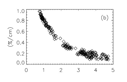
It can be seen that this is a non linear relationship; the thickness of the ice cover is determined by its winter thickness, as that thins the amount of water exposed by a given melt increases until March thickness is only around 1m by which time 100cm of seasonal melt exposes 100% of the ocean. As shown in my previous post, in the PIOMAS model the seasonal loss of thickness is increasing in the American and Siberian sectors, and for all three sectors the thickness in April and September is decreasing. So not only is OWFE changing due to increasing open water, but over most of the pack PIOMAS thinning during the melt season is increasing.
What drives the shape of this plot? In early years thick ice can experience large changes in thickness without a resultant change in OWFE because the seasonal melt is nowhere near 3 to 5 metres and open water is therefore not exposed, which means the slope is shallow. At the end of the series, April thickness nears the melt required to make 100% open water, so even a slight trend in thinning has a large effect on open water formation. And between these two extremes as the ice pack thins we have a gradual increase in the efficacy of open water production by seasonal melt as the ice pack thins.
I've calculated OWFE for all three regions as defined in my previous post, this uses the same definition of OWFE as in Holland et al. As stated in my previous post, percentage open water in September is calculated with respect to the preceding April's sea ice area within the region concerned. April thickness is calculated as the total of April grid box volumes in the region concerned divided by the total area of ice (adjusted using concentration) within the region concerned.
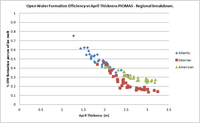
Fig 2, OWFE as a function of April thickness from PIOMAS for each individual region, north of 65degN latitude.
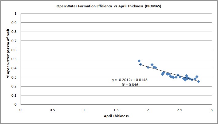
Fig 3, OWFE as a function of April thickness from PIOMAS for the whole region north of 65degN latitude (Whole Arctic).

Fig 4, Key indicators used in figure 3, including for comparison % Open Water as calculated from Cryosphere Today, using 10M km^2 as the reference (maximum) ice cover. Sea ice thickness on left side vertical axis, % open water on right side.
It may seem at first glance that the OWFE plot for the whole Arctic is linear, but it starts and ends above the linear trend line whilst dropping below the trend in the middle, so it is showing the same behaviour as figure 1, it is just earlier in the process than much of figure 1. Being the sum of the three sets in figure 2, figure 3 shows a lesser range, particularly in terms of OWFE (%open water per cm of melt), this is because the behaviour in the Atlantic sector is weighted out by the far larger areas of the American and Siberian sectors combined. (I know it looks like I've left out Atlantic, but before clicking publish I've just checked my code for what must be the fourth time, and I haven't)
However the OWFE clearly shows the same sort of behaviour found in the model runs studied by Holland et al. As the ice thins (loses volume) the ease with which open water can be revealed increases, with consequent ice albedo feedback and autumn heat loss. Loss of volume and loss of area are not unrelated, they are intrinsically connected by OWFE, the volume loss and resultant loss of thickness drives the loss of area/extent. This is not to say they are the only factors. In the Siberian and American sectors the amount of thinning has increased this century, I see several reasons for this; increasing shift to first year ice with attendant drop in albedo, the Arctic Dipole anomaly, and possibly increased ocean heat flux. The Atlantic sector's lack of increase in melt rate may seem to argue against that latter issue. However the Atlantic sector includes both the Barents and Kara seas, where Atlantic Ocean heat flux can directly affect the ice, and the region further west down towards Svalbard and the Fram Strait, where a combination of Atlantic water dropping out of contact with the ice, and influx of new ice could be the reason for the lack of increase in seasonal melt.
There is another reason to look at ocean heat flux, because Holland et al find that the Rapid Ice Loss Events (RILEs) they're studying in models are thermodynamically driven, with factors such as transport and ridging of ice not playing a major role. In particular they find that the RILEs follow influxes of warm ocean water, with regrowth of ice causing brine formation, which drops drawing in warmer waters through Bering and the Atlantic sector. It is conceivable that such a process is going on in recent autumns and may actually be bringing the deeper Atlantic water under the Arctic Ocean into some form of interaction with the ice. Overland et al's recent finding of an early summer Arctic Dipole (see here) also has the potential to draw warmer water in through the Bering Strait. And in the extremely low sea ice area in Barents recently may be indicative of an influx of warm Atlantic waters.
However it worth keeping things in perspective, the change in albedo caused by the change from young to old ice increases sunlight absorption by 1/3, this implies an increase of over 30W/m^2 from June to September for each square metre that converts from old ice to young ice. This is much bigger factor than any similar figures I've seen for ocean heat factors, and of course it (and the Arctic Dipole impacts) are thermodynamic impacts.
Hidden in figure 1 there are also Rapid Ice Loss Events (RILEs). Holland et al identify RILEs as explained in the following passage.
In the period since 1979, both in terms of extent and area, this criterion is not met at any time. I've used NSIDC extent and CT area and calculated the 5 year (current year and four previous years) running mean for the September mean, then taken the year to year difference as the derivative of that 5 year running mean, the result is shown in figure 5 below. At no point does the result exceed 0.5M km^2.We identify an abrupt event when the derivative of the five-year running mean smoothed September ice extent timeseries exceeds a loss of 0.5 million km2 per year, equivalent to a loss of 7% of the 2000 ensemble mean ice extent in a single year.
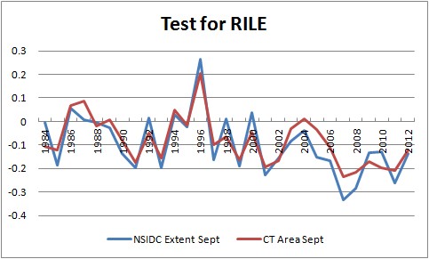
Fig 5, derivative of 5 year running mean, area and extent, see above text.
So does this mean I don't think we're in a RILE? I've been aware of this paper for some years, and knowing that current circumstances don't fit the model defined RILE hasn't stopped me from concluding that we are in one.
Figure 2b of Holland et al is shown in figure 1 above. Here is figure 2a.
The grey band shows the RILE that passes the test outlined above. However there is another large drop before that, just after 2000 at just under 3m thickness. So we have two drops, around just under 3m and just under 2m March thickness. Now referring to figure 1 it can be seen that these drops appear in the OWFE/March thickness plot as spacings in the scatterplot. A crucial point to note here is that not only are these spacings due to change in thickness (horizontal movement), they also involve vertical movement, which implies an increase of OWFE at these times. The CCSM3 model run starts with a much larger thickness then PIOMAS, so direct comparison with the PIOMAS data isn't straightforward. However this gap formation in the OWFE plot seems to be a reasonable way to look for a RILE type event, Holland et al's strict definition seems to have missed a RILE in figure 6, and event that examination of figure 1 shows is very similar to the one their criteria picks up.
Figure 5, the test for a RILE used by Holland et al, and applied to observational data shows that post 2007 behaviour is unusually negative. If I am correct and we are in the start of a RILE then this should become more negative. However figure 3, my calculation of OWFE/April Thickness, seems to show the same spreading observed in figure 1 from Holland et al. In the PIOMAS data we have two April thickness drops, which when used as a function of OWFE reveal gaps: 2012 and 2011 are together, then 2009 to 2007 are in another groups, with preceding years forming a contiguous spread. Once again, both gaps involve not only horizontal shifting due to loss of April thickness, they also involve vertical shifting due to increased OWFE.
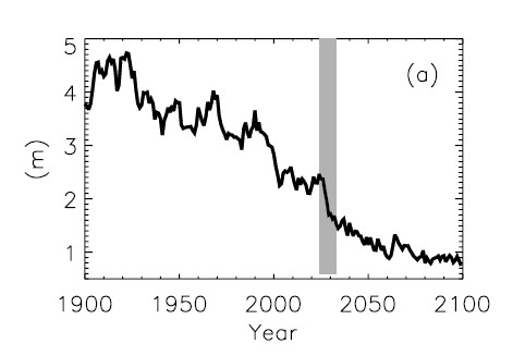
It's worth considering what the graph of OWFE as a function of April thickness will look like in years to come. So far we have 34 years in the series that makes up figure 2 and 3, I expect that percentage open water will approach 100% by as early as 2020, feasibly sooner, this would cause a persistent thinning of the data points in figure, unlike the model considered by Holland et al, which has a long tail of persistent remaining sea ice (figure 6) which causes a reclustering as the curve proceeds towards an OWFE of 1.
So we have 34 past data points, how many will it take to reach 100% open water? Figure 4 implies that a meeting point between average April thickness and average thinning is imminent. But rather than get lost in the complication of what a surviving core of thick ice means for that, let's cut straight to volume.
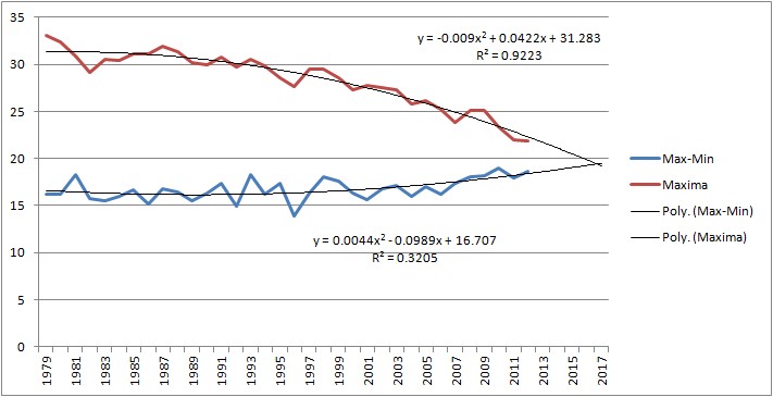
Fig 7, Plot of maximum volume minus minimum volume (seasonal losses) and maximum volume (daily figures 1000 km^3), with extrapolation of naive trends.
Figure 7 has been done by others elsewhere. But I wanted to produce my own version to put the question of the future trajectory of figure 3 (OWFE vs April thickness) into context. Combining figure 7 and the open water formation behaviour described in figures 1, 2 and 3 suggests to me that we will see massive year on year losses of area within a few years. Because figures 4 and 7 (average thickness and volumes) imply that net season thinning is closely approaching net maximum thickness and the curve of figure 1 (Holland et al) applied to figure 3 (PIOMAS OWFE vs April Thickness) will take care of the massive area reduction.
If there is something that's going to stop the loss of volume, I can't figure it out. If PIOMAS is wildly wrong, I can't see why.
8 comments:
If the thickness is a meter then for 100 cm of melt, OW is going to result so it is not surprising that OWFE reaches 100% at 1m.
I am wondering if this is a sensible measure.
Last year we had 18.6 K Km^3 volume reduction and area at time of volume maximum was 12.93 m km^3. This implies average thickness melt of 1.44m. As there is lots of thin areas with less than 1.44m thickness at the volume max, then the melt season would seem likely to melt any cell with 1.5m or less ice.
Therefore should we have some form of OWFE measure that approaches 100% at a thickness of 1.5m rather than at 1m?
If we calculated sum of ((lower of Piomas thickness and 1.5)*cell area) for April of each year. How would that differ from volume reduction in that year?
Perhaps find the figure which if used instead of 1.5 makes the volume reduction correct and see how that figure changes.
Could this better predict the volume reduction?
Not sure if these numbers are interesting: (hope formatting isn't too bad)
Year 2010, Apr Avg Thick, Reduction, Sept Avg Thick, No cells
Sept lt 10cm, 1.138800989, 1.133596751, 0.005204238, 10768
Sept gt 10cm, 2.251138011, 1.230686617, 1.020451395, 6731
Year 2012, Apr Avg Thick, Reduction, Sept Avg Thick, No cells
Sept lt 10cm, 1.174049807, 1.16953493, 0.004514878, 12245
Sept gt 10cm, 2.304140099, 1.210651578, 1.093488521, 5289
The thinning of cells going to 0 thickness seems surpisingly similar to thinning of cells that retain some thickness. I guess that is just co-incidence with thinning of cells in center of (MYI?) pack and outside edges being lower than maximum thinning cells and it just happens to average out.
BTW, Have you got a csv file of latest cell areas in same order as heff files?
Correction in 2012 there are 11245 cell with Sept thickness less than 10cm.
By deciles (1653 cells) 2012 thinning was:
Apr Thick, Reduction, Sept Thick
0.058553478, 0.058553478, 0
0.572480337, 0.572480337, 0
1.122923139, 1.122923139, 0
1.601478836, 1.601478836, 0
2.087651403, 2.087651402, 4.43247E-10
1.317933088, 1.317448419, 0.000484669
1.548861945, 1.492142027, 0.056719918
1.930705475, 1.470039892, 0.460665583
2.220763057, 1.142817656, 1.077945402
2.895054369, 0.961668537, 1.933385831
Maximum thinning decile has over 2m of melt! If the pack was all 2m thick would it all melt? I don't think so, because those will be cells that get to be on the edge of the pack and get melted at a fast rate. Also some cells will be related to transport out of ice. Does that affect as much as 10% of cells? Hmm not sure. Even if there is a decile of transport then the next decile going to 0 thickness shows 1.6m melt. That is a substantial thickness that can melt out.
3m ice suffers less than 1m of thinning. Again some (but not as much) could be transport but more likely the 3m ice is MYI that is difficult to melt as well as not being thin to reduce albedo as it gets thinner. Still get 1m of thinning compared to 1.6m so it isn't hugely harder to melt.
I wouldn't get too hung up on the 100% 1m issue. It's not mentioned in the paper but I can't see any good reason why one couldn't have a short period at the end of the summer without ice at average thickness (April) of 1.5m and average thinning of 1.5m leading to open water of 100% i.e. OWFE = 100/150 = 0.666...
In that case the scatter plot wouldn't reach 1 before 100% open water occurred.
Actually there may be a good reason - thicker ice inside the pack and more thinning at the edges. Another that's just occurred to me is that we're talking about monthly averages, not just a few days of 100% OW.
This is why I did my first post using %OW as opposed to Holland et al's defined OWFE.
I've just been so concerned I might have screwed up again that I checked the source paper: They state - "defined as the percent open water formation
per cm of ice melt over the melt season"
Perhaps a better metric would be to replace cm of melt over the melt season with 'melt over the melt season expressed as a percentage of April thickness'. Off the top of my head I think that might consistently normalised to zero. But should keep the general form of the scatter.
As usual you get complex very fast, I've just got in from work and need a meal and a rest before considering the rest of what you say.
Crandles,
Sorry but I've just had a call and need to start work tomorrow at 0400, so I'm going to have a night off tonight and get back to you tomorrow.
Isn't Wipneus's spreadsheet of grid areas in the correct order? If not I can easily copy Rob's into the necessary order.
PS tried out what I suggested re referencing melt to April thickness, not what I was expecting.
No rush. Not sure my thoughts are going anywhere either on OWFE measure or the decile analysis I have been trying.
4am start and 12 hour day are tiring, hope it went OK.
Yep, fine. Got today off but still not firing on all cylinders. Leaving aside the OWFE issue for here, I see you've been moving forward with your thickness/melt vulnerability idea. I'll 'meet you' over at Neven's to discuss that.
I am probably just not getting my heat around OWFE%.
I think your division of NH into 3 areas is reasonable as the area go all the way to North Pole.
If you tried applying measure to a region like Kara which had 40cm thickness and reached 100% open water the OWFE% calculates to 250%.
What does 250% mean???
If we could actually melt 1.5m of ice then perhaps 375% might be a more sensible answer.
It seems the measure is not appropriate for areas that completely melt out. Maybe the measure should only be used to compare the same areas at different date. So comparing different area is a bit dodgy?
I am struggling to work out what sort of measure I am grasping for.
I am probably just not getting my head around it and this is a problem with me rather than a problem for you.
Post a Comment